BuzzTech: Machine Learning at the Edge: Deploying YOLOv8 on Raspberry Pi Zero 2W for Real-Time Bee Counting at the Hive Entrance

Introduction

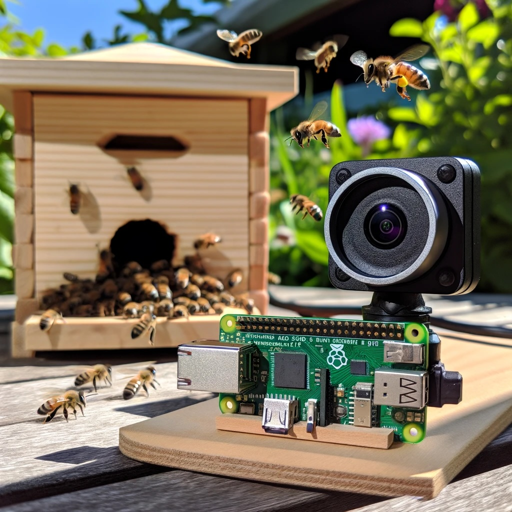
At the Federal University of Itajuba in Brazil, with the master's student José Anderson Reis and Professor José Alberto Ferreira Filho, we are exploring a project that delves into the intersection of technology and nature. This tutorial will review our first steps and share our observations on deploying YOLOv8, a cutting edge machine learning model, on the compact and efficient Raspberry Pi Zero 2W (Raspi-Zero). We aim to estimate the number of bees entering and exiting their hive—a task crucial for beekeeping and ecological studies

Why is this important? Bee populations are vital indicators of environmental health, and their monitoring can provide essential data for ecological research and conservation efforts. However, manual counting is labor-intensive and prone to errors. By leveraging the power of embedded machine learning, or tinyML, we automate this process, enhancing accuracy and efficiency.

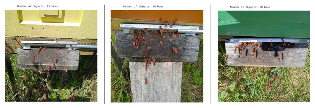
This tutorial will cover setting up the Raspberry Pi, integrating a camera module, optimizing and deploying YOLOv8 for real-time image processing, and analyzing the data gathered.

Installing and using Ultralytics YOLOv8

Ultralytics YOLOv8, is a version of the acclaimed real-time object detection and image segmentation model, YOLO. YOLOv8 is built on cutting-edge advancements in deep learning and computer vision, offering unparalleled performance in terms of speed and accuracy. Its streamlined design makes it suitable for various applications and easily adaptable to different hardware platforms, from edge devices to cloud APIs.

Let's start installing the Ultarlytics packages for local inference on the Rasp-Zero:

1. Update the packages list, install pip, and upgrade to the latest:

sudo apt update
sudo apt install python3-pip -y
pip install -U pip

1. Install the ultralytics pip package with optional dependencies:

pip install ultralytics

1. Reboot the device:

 sudo reboot

Testing the YOLO

After the Rasp-Zero booting, let's create a directory for working with YOLO and change the current location to it:

mkdir Documents/YOLO
cd Documents/YOLO

Let's run inference on an image that will be downloaded from the Ultralytics website, using the YOLOV8n model (the smallest in the family) at the Terminal (CLI):

yolo predict model=yolov8n-seg.pt source='https://ultralytics.com/images/bus.jpg' imgsz=640

The inference result will appear in the terminal:

In the image (bus.jpg), 4 persons , 1 bus, and 1 stop signal were detected:

Also, we got a message that:

Results saved to runs/detect/predict4 .

Inspecting that directory, we can see a new image saved (bus.jpg). Let's download it from the Rasp-Zero to our desktop for inspection:

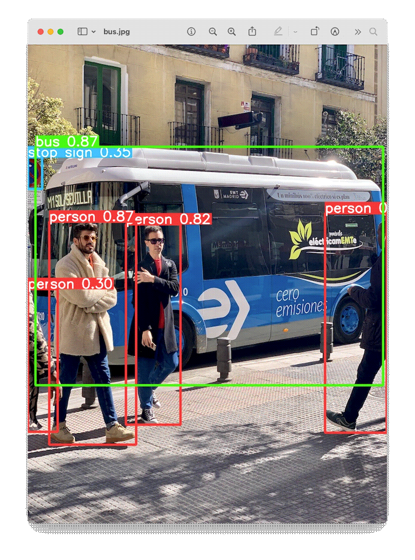
So, the Ultrayitics YOLO is correctly installed on our Rasp-Zero.

Export Model to NCNN format

An issue is the high latency for this inference,  7.6 s, even with the smaller model of the family (YOLOv8n). This is a reality of deploying computer vision models on edge devices with limited computational power, such as the Rasp-Zero. One alternative is to use a format optimized for optimal performance. This ensures that even devices with limited processing power can handle advanced computer vision tasks well.

Of all the model export formats supported by Ultralytics, the NCNN is a high-performance neural network inference computing framework optimized for mobile platforms. From the beginning of the design, NCNN was deeply considerate about deployment and use on mobile phones and did not have third-party dependencies. It is cross-platform and runs faster than all known open-source frameworks (such as TFLite).

NCNN delivers the best inference performance when working with Raspberry Pi devices. NCNN is highly optimized for mobile embedded platforms (such as ARM architecture).

So, let's convert our model and rerun the inference:

1. Export a YOLOv8n PyTorch model to NCNN format, creating:  '/yolov8n_ncnn_model'

yolo export model=yolov8n.pt format=ncnn

2. Run inference with the exported model (now the source could be the bus.jpg image that was downloaded from the website to the current directory on the last inference):

yolo predict model='./yolov8n_ncnn_model' source='bus.jpg'

Now, we can see that the latency was reduced by half.

Estimating the number of Bees

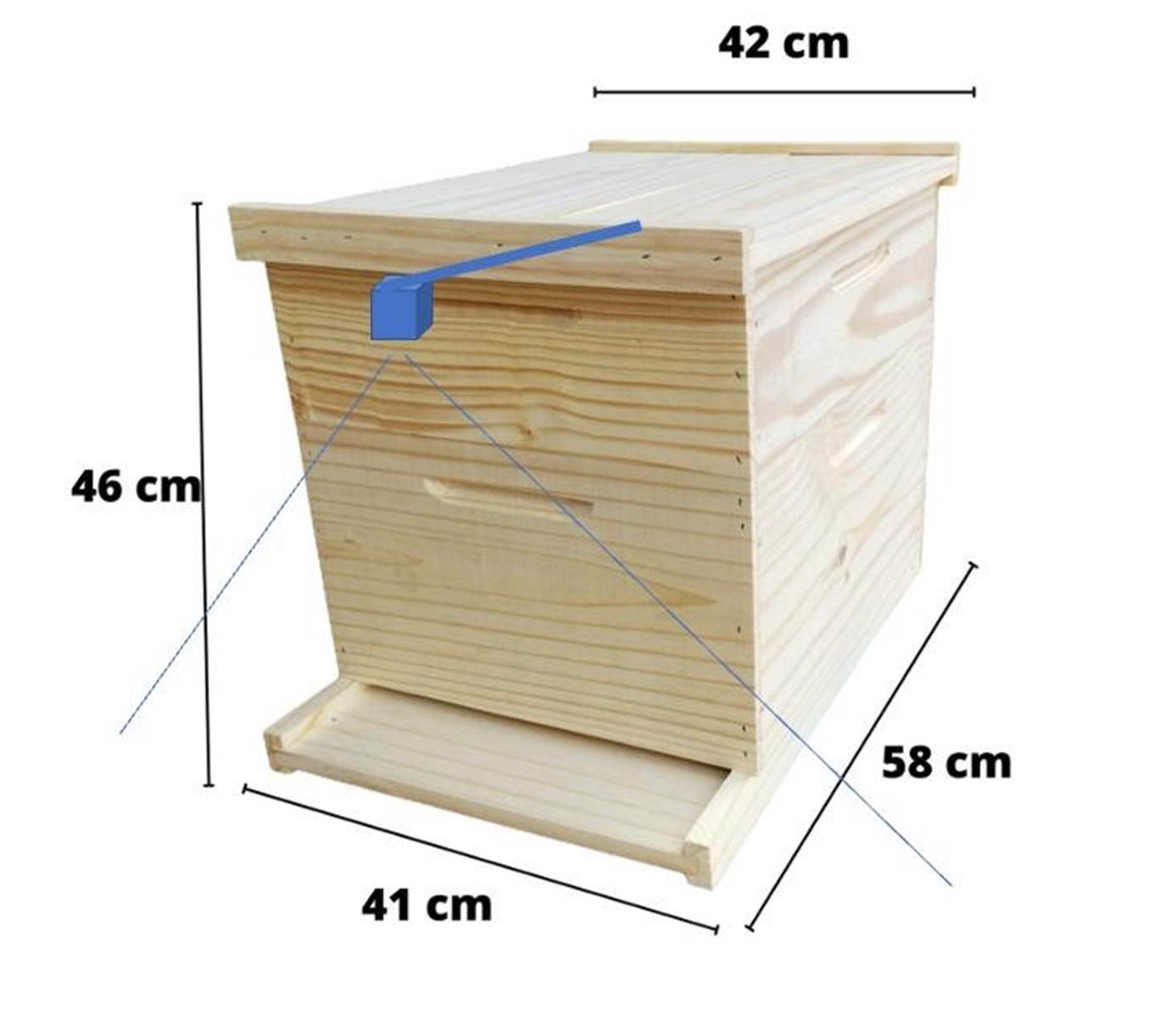
For our project at the university, we are preparing to collect a dataset of bees at the entrance of a beehive using the same camera connected to the Rasp-Zero. The images should be collected every 10 seconds. With the Arducam OV5647, the horizontal Field of View (FoV)  is 53.5o, which means that a camera positioned at the top of a standard Hive (46 cm) will capture all of its entrance (about 47 cm).

Dataset

The dataset collection is the most critical phase of the project and should take several weeks or months. For this tutorial, we will use a public dataset: "Sledevic, Tomyslav (2023), “[Labeled dataset for bee detection and direction estimation on beehive landing boards,” Mendeley Data, V5, doi: 10.17632/8gb9r2yhfc.5"

The original dataset has 6,762 images (1920 x 1080), and around 8% of them (518) have no bees (only background). This is very important with Object Detection, where we should keep around 10% of the dataset with only background (without any objects to be detected).

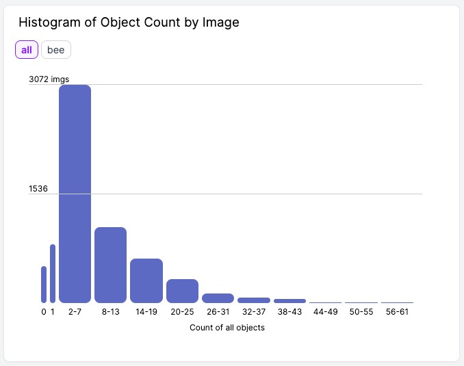
The images contain from zero to up to 61 bees:

We downloaded the dataset (images and annotations) and uploaded it to Roboflow. There, you should create a free account and start a new project, for example, (Bees_on_Hive_landing_boards):

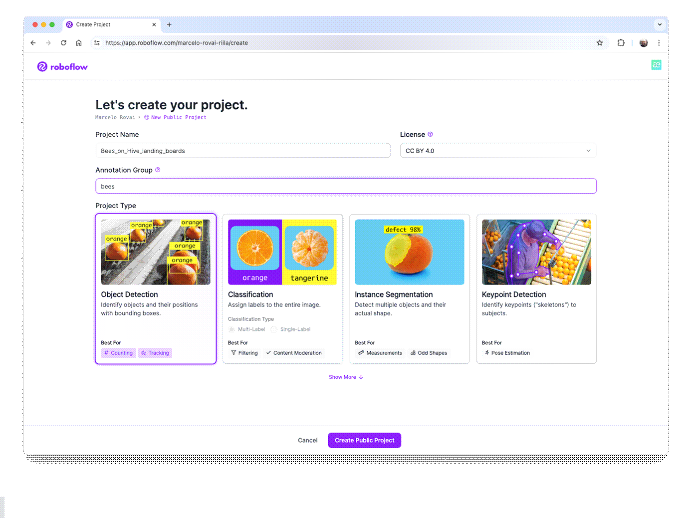We will not enter details about the Roboflow process once many tutorials are available.

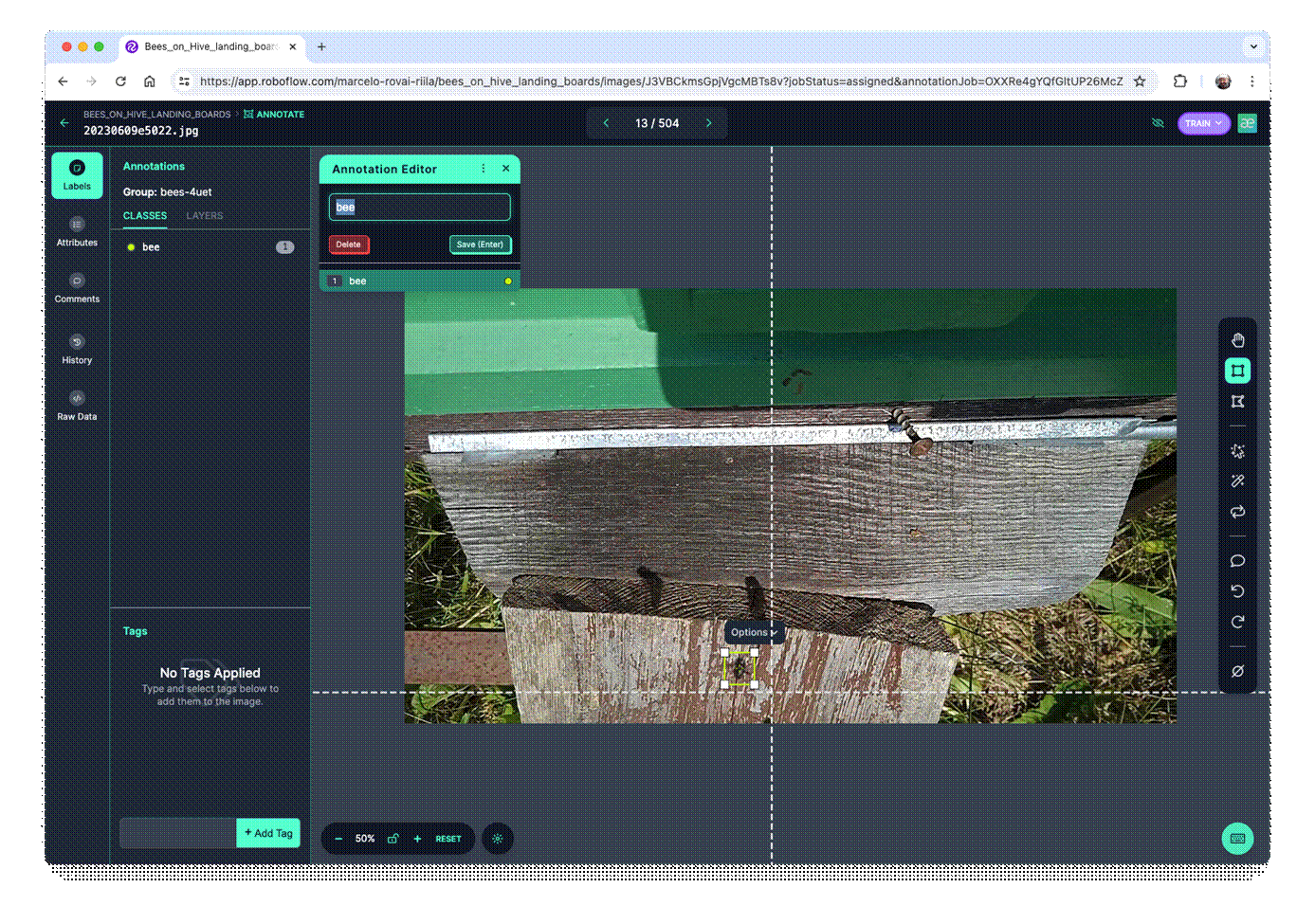
Once the project is created and the dataset is uploaded, you should review the annotations using the "AutoLabel" Tool. Note that all images with only a background should be saved w/o any annotations. At this step, you can also add additional images.

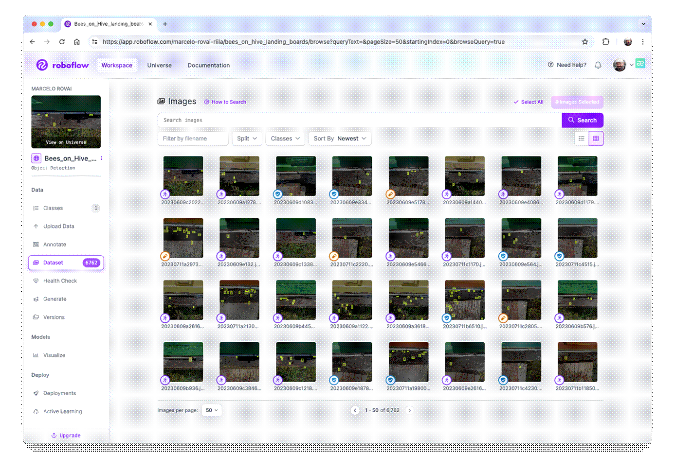
Once all images are annotated, you should split them into training, validation, and testing.

Pre-Processing

The last step with the dataset is preprocessing to generate a final version for training. The Yolov8 model can be trained with 640 x 640 pixels (RGB) images. Let's resize all images and generate augmented versions of each image (augmentation) to create new training examples from which our model can learn.

For augmentation, we will rotate the images (+/-15o) and vary the brightness and exposure.

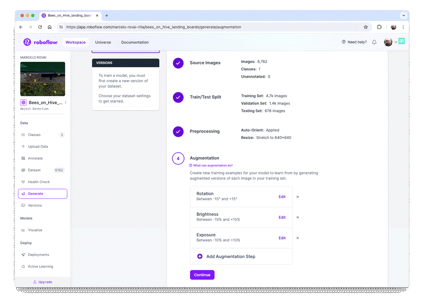
This will create a final dataset of 16,228 images.

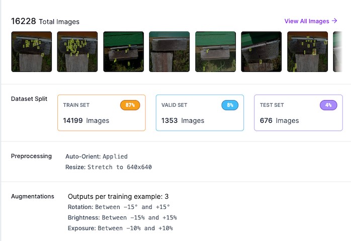
Now, you should export the model in a YOLOv8 format. You can download a zipped version of the dataset to your desktop or  get a downloaded code to be used with a Jupyter Notebook:

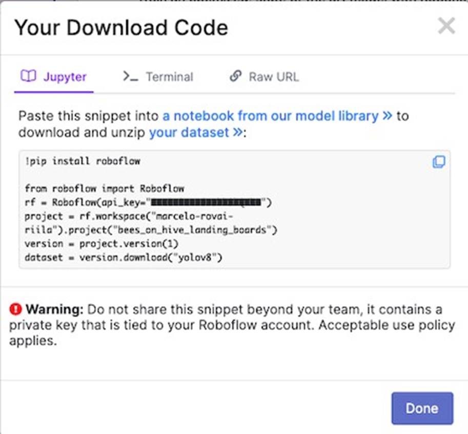
And that is it! We are prepared to start our training using Google Colab.

The pre-processed dataset can be found at the Roboflow site.

Training YOLOv8 on a Customized Dataset

For training, let's adapt one of the public examples available from Ultralitytics and run it on Google Colab:

           yolov8_bees_on_hive_landing_board.ipynb Open in Colab

Critical points on the Notebook:                       

5.     Define the main hyperparameters that you want to change from default, for example:

6.     Run the training (using CLI):

7.     Note that the trained model ( best.pt ) is saved in the folder  /runs/detect/train3/weights/ . Now, you should validade the trained model with the valid/images .

!yolo task=detect mode=val model={HOME}/runs/detect/train3/weights/best.pt data=

{dataset.location}/data.yaml

The results were similar to training.

8.     Now, we should perform inference on the images left aside for testing

We can also perform inference with a completely new and complex image from another beehive with a different background (the beehive of Professor Maurilio of our University). The results were great (but not perfect and with a lower confidence score). The model found 41 bees.

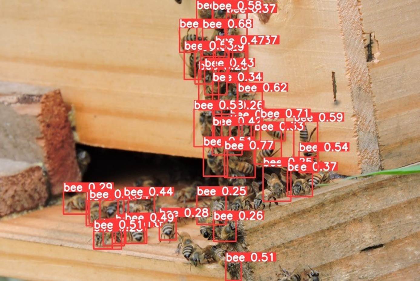
9.     The last thing to do is export the train, validation, and test results for your Drive at Google. To do so, you should mount your drive.

Inference with the trained model, using the Rasp-Zero

Using the FileZilla FTP, let's transfer the best.pt to our Rasp-Zero (before the transfer, you may change the model name, for example, bee_landing_640_best.pt ).

The first thing to do is convert the model to an NCNN format: yolo export model=bee_landing_640_best.pt format=ncnn

As a result, a new converted model, bee_landing_640_best_ncnn_model is created in the same directory.

Let's create a folder to receive some test images (under Documents/YOLO/ :

Using the FileZilla FTP, let's transfer a few images from the test dataset to our Rasp-Zero:

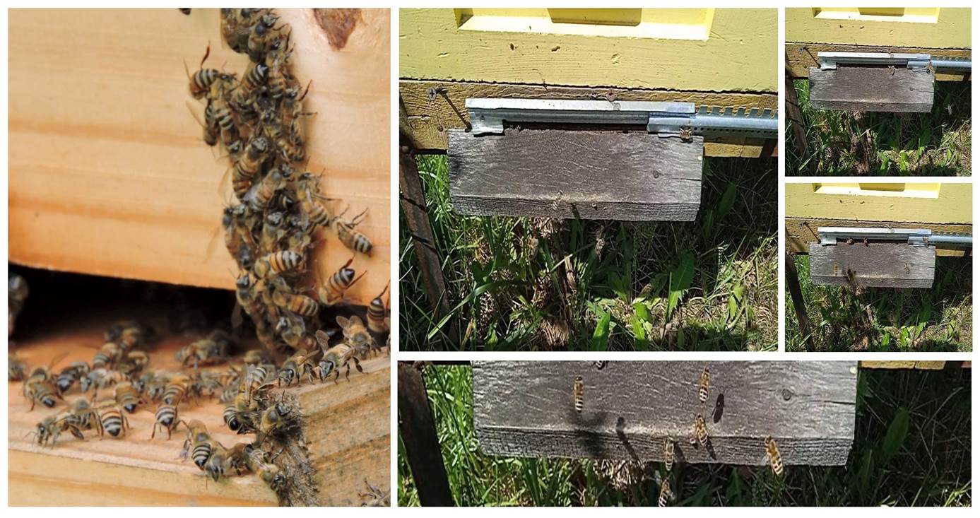
Let's use the Python Interpreter:

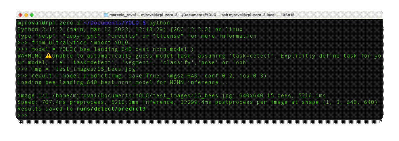
As before, we will import the YOLO library and define our converted model to detect bees:

Now, let's define an image and call the inference (we will save the image result this time to external verification):

img = 'test_images/15_bees.jpg'

result = model.predict(img, save=True, imgsz=640, conf=0.2, iou=0.3)

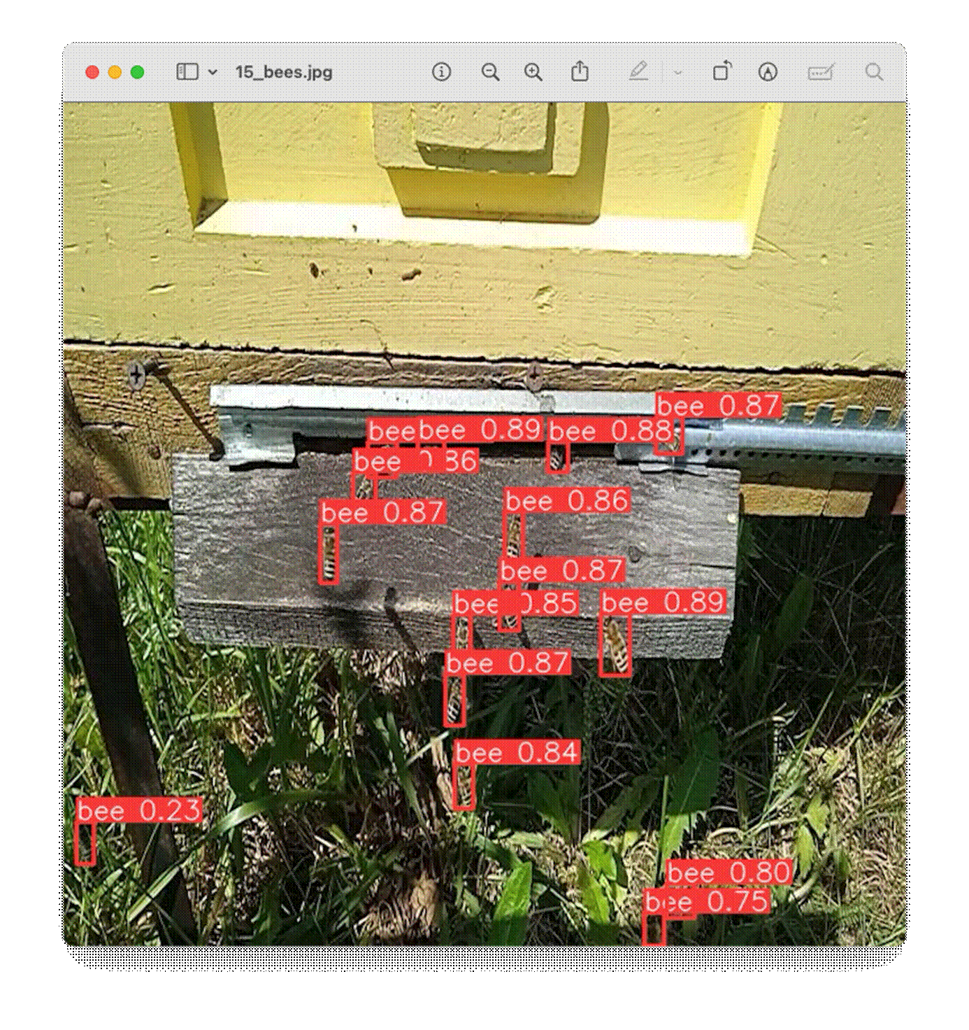
The inference result is saved on the variable result, and the processed image on runs/detect/predict9

Using FileZilla FTP, we can send the inference result to our Desktop for verification:

let's go over the other images, analyzing the number of objects (bees) found:

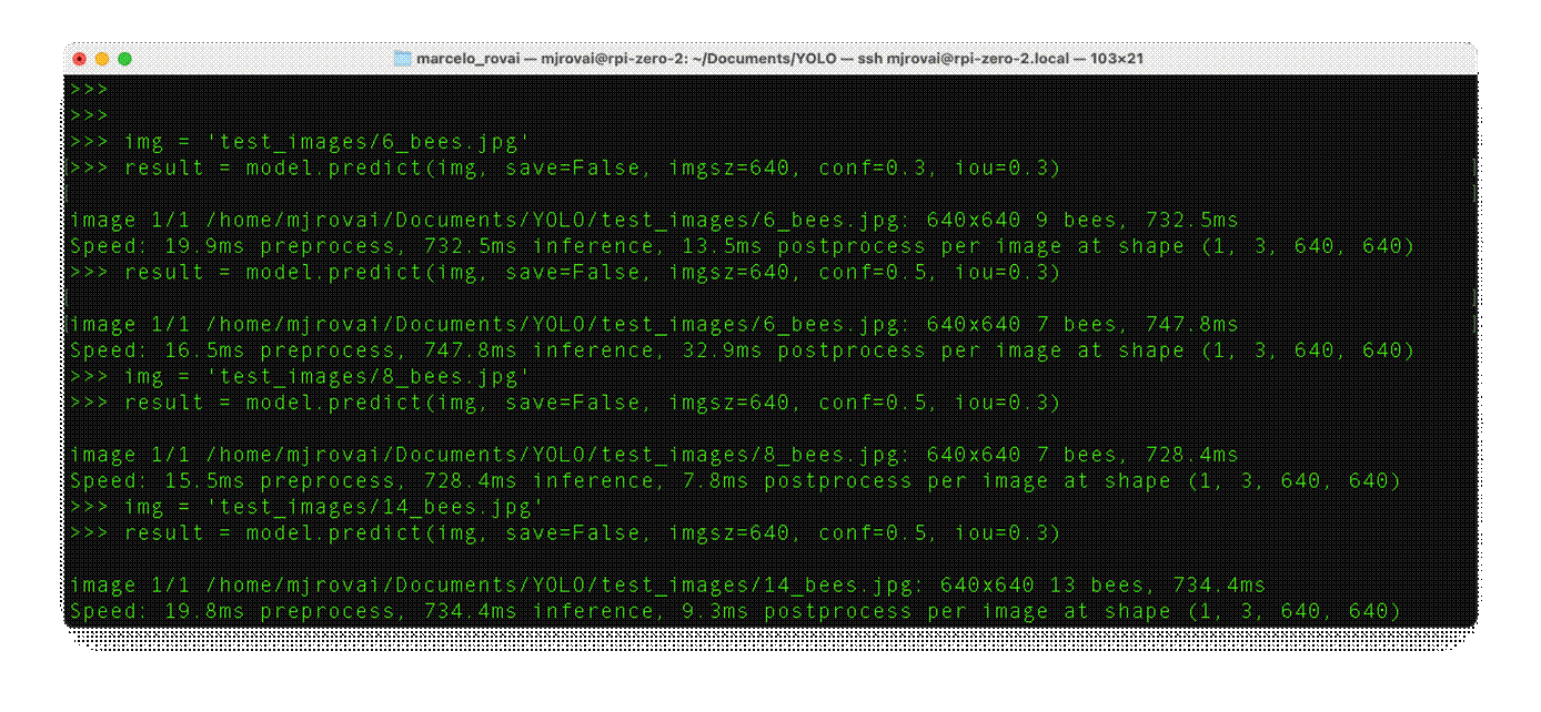
Depending on the confidence, we can have some false positives or negatives. But in general, with a model trained based on the smaller base model of the YOLOv8 family (YOLOv8n) and also converted to NCNN, the result is pretty good, running on an Edge device such as the Rasp-Zero. Also, note that the inference latency is around 730ms.

For example, by running the inference on Maurilio-bee.jpeg , we can find 40 bees . During the test phase on Colab,  41 bees were found (we only missed one here.)

Considerations about the Post-Processing

Our final project should be very simple in terms of code. We will use the camera to capture an image every 10 seconds. As we did in the previous section, the captured image should be the input for the trained and converted model. We should get the number of bees for each image and save it in a database (for example, timestamp: number of bees).

We can do it with a single Python script or use a Linux system timer, like cron , to periodically capture images every 10 seconds and have a separate Python script to process these images as they are saved. This method can be particularly efficient in managing system resources and can be more robust against potential delays in image processing.

Setting Up the Image Capture with cron  

First, we should set up a cron job to use the rpicam-jpeg command to capture an image every 10 seconds.

1.     Edit the crontab :

Open the terminal and type crontab -e to edit the cron jobs.

cron normally doesn't support sub-minute intervals directly, so we should use a workaround like

a loop or watch for file changes.

2.     Create a Bash Script ( capture.sh ):

   Image Capture: This bash script captures images every 10 seconds using rpicam-jpeg , a command that is part of the raspijpeg tool. This command lets us control the camera and capture JPEG images directly from the command line. This is especially useful because we are looking for a lightweight and straightforward method to capture images without the need for additional libraries like Picamera or external software. The script also saves the captured image with a timestamp.

Setting Up the Python Script for Inference     

Image Processing: The Python script continuously monitors the designated directory for new images, processes each new image using the YOLOv8 model, updates the database with the count of detected bees, and optionally deletes the image to conserve disk space.

Database Updates: The results, along with the timestamps, are saved in an SQLite database. For that, a simple option is to use sqlite3.

In short, we need to write a script that continuously monitors the directory for new images, processes them using a YOLO model, and then saves the results to a SQLite database. Here’s how we can create and make the script executable:

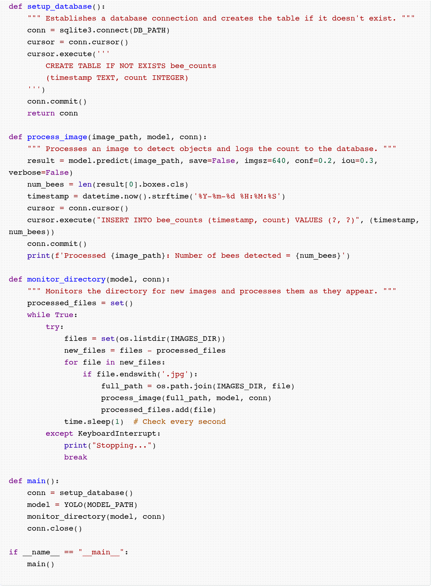
The python script must be executable, for that:

1.     Save the script: For example, as process_images.py .

2.     Change file permissions to make it executable:

or

Note that we are capturing images with their own timestamp and then log a separate timestamp for when the inference results are saved to the database. This approach can be beneficial for the following reasons:

1.     Accuracy in Data Logging:

   Capture Timestamp: The timestamp associated with each image capture represents the exact moment the image was taken. This is crucial for applications where precise timing of events (like bee activity) is important for analysis.

   Inference Timestamp: This timestamp indicates when the image was processed and the results were recorded in the database. This can differ from the capture time due to processing delays or if the image processing is batched or queued.

2.     Performance Monitoring:

   Having separate timestamps allows us to monitor the performance and efficiency of your image processing pipeline. We can measure the delay between image capture and result logging, which helps optimize the system for real-time processing needs.

3.     Troubleshooting and Audit:

   Separate timestamps provide a better audit trail and troubleshooting data. If there are issues with the image processing or data recording, having distinct timestamps can help isolate whether delays or problems occurred during capture, processing, or logging.

Script For Reading the SQLite Database

Here is an example of a code to retrieve the data from the database:

#!/usr/bin/env python3
import sqlite3
def main():
  db_path = 'bee_count.db'
  conn = sqlite3.connect(db_path)
  cursor = conn.cursor()
  query = "SELECT * FROM bee_counts"
  cursor.execute(query)
  data = cursor.fetchall()
  for row in data:
  print(f"Timestamp: {row[0]}, Number of bees: {row[1]}")
  conn.close()
if __name__ == "__main__":
  main()

Adding Environment data

Besides bee counting, environmental data, such as temperature and humidity, are essential for monitoring the bee-have health. Using a Rasp-Zero, it is straightforward to add a digital sensor such as the DHT-22 to get this data.

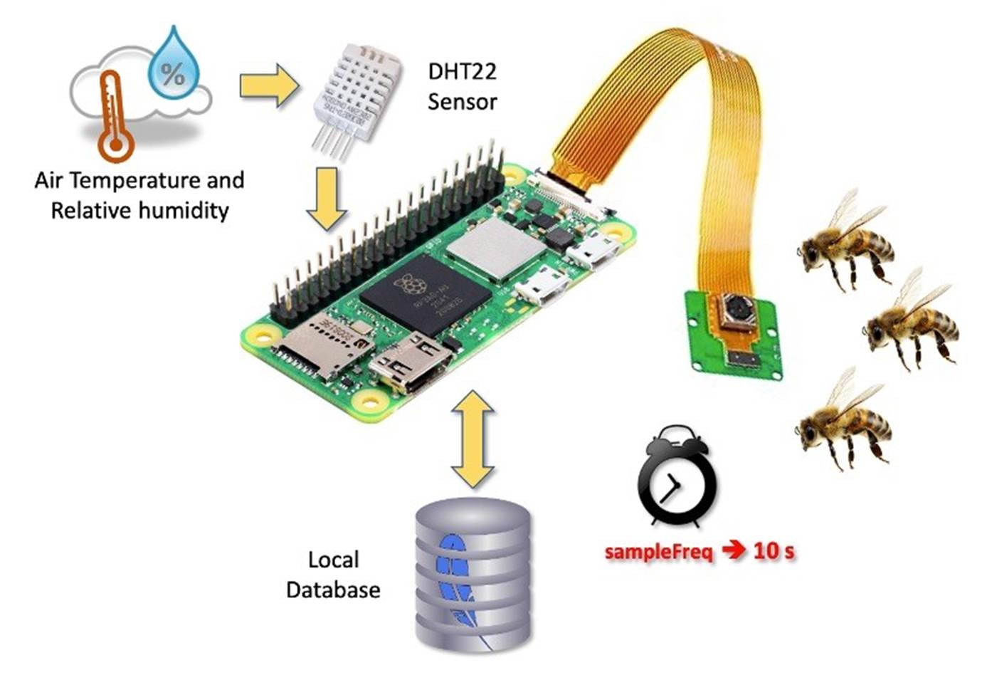
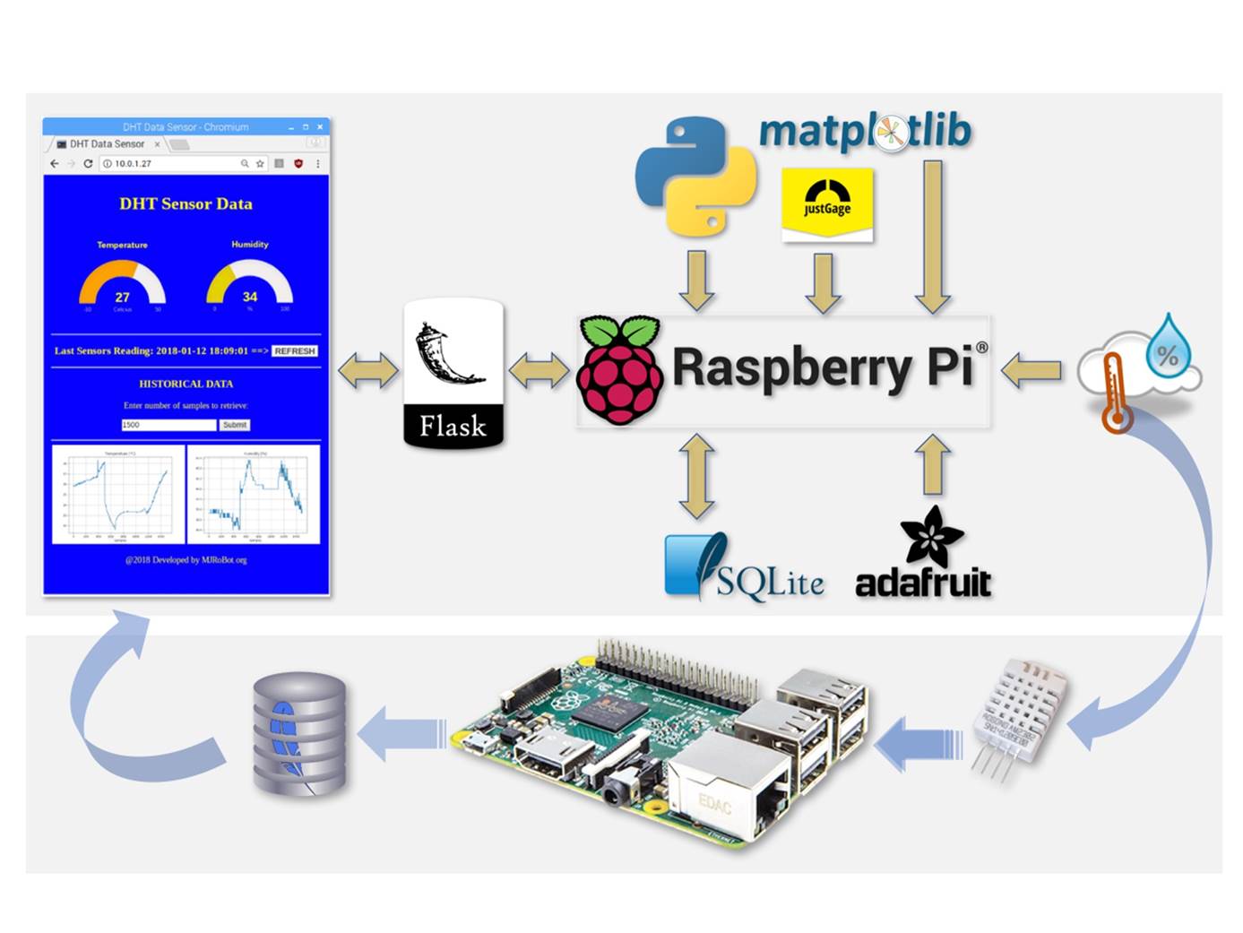
Environmental data will be part of our final project. If you want to know more about connecting sensors to a Raspberry Pi and, even more, how to save the data to a local database and send it to the web, follow this tutorial: From Data to Graph: A Web Journey With Flask and SQLite.

Conclusion

In this tutorial, we have thoroughly explored integrating the YOLOv8 model with a Raspberry Pi Zero 2W to address the practical and pressing task of counting (or better, "estimating") bees at a beehive entrance. Our project underscores the robust capability of embedding advanced machine learning technologies within compact edge computing devices, highlighting their potential impact on environmental monitoring and ecological studies.

This tutorial provides a step-by-step guide to the practical deployment of the YOLOv8 model. We demonstrate a tangible example of a real-world application by optimizing it for edge computing in terms of efficiency and processing speed (using NCNN format). This not only serves as a functional solution but also as an instructional tool for similar projects.

The technical insights and methodologies shared in this tutorial are the basis for the complete work to be developed at our university in the future. We envision further development, such as integrating additional environmental sensing capabilities and refining the model's accuracy and processing efficiency.

Implementing alternative energy solutions like the proposed solar power setup will expand the project's sustainability and applicability in remote or underserved locations.

The Dataset paper, Notebooks, and PDF version are in the Project repository.

On the Tiny ML4D website, you can find lots of educational materials on TinyML. They are all free and opensource for educational uses—we ask that if you use the material, please cite it! TinyML4D is an initiative to make TinyML education available to everyone globally.